Projects
This is where I put any supplementary materials and resources I use in my work. I primarily use this page to showcase Sage and/or jupyter notebook files I use as proof of concept, tutorials, or models for dynamical systems. The website provides instructions on how to get Sage up and running on your system. I also provide pdf/html exports of most of these notebooks that anyone can view, I'll attach them below.
Deep Learning Kernel Functions (Interactive HTML | Jupyter Notebook)
This deep learning framework is made entirely in PyTorch 2.1.1 and makes use of a suite of different symbolic differentiation tools to produce these Neural Networks. I introduce some of the constraints we need to make on weights and quickly justify why these assumptions ensure we're truly getting initial laws and Markov kernels. View the HTML link above for a more detailed treatment of kernels, generalizations of kernels, and applications.
Consider the measure space \( (\mathcal{X},\mathcal{F},m)\). A Markov kernel function is a function
that is measurable in both coordinates such that
is a probability measure for every \(x\in \mathcal{X}\) and for every \(A\in \mathcal{F}\),
is a measureable function. An initial law is a probability measure \(\mu:\mathcal{F}\to [0,1]\) such that the distribution of an initial random variable \(X_0\) is distributed according to \(\mu\). A Markov chain \(X_0,X_1,...\) is a sequence of random variables that satisfies the Markov condition:
for all \(A\in \mathcal{F}\). If we know a chain's values up until $x_{n-1}$, the conditional probability of the next state is dependent only on the previous state.
A Markov chain can be modeled using a kernel by taking
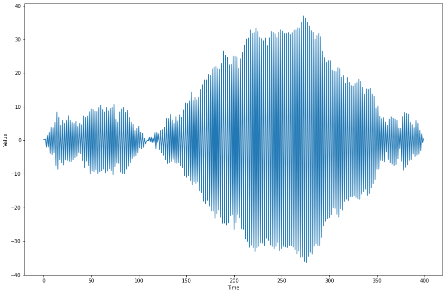
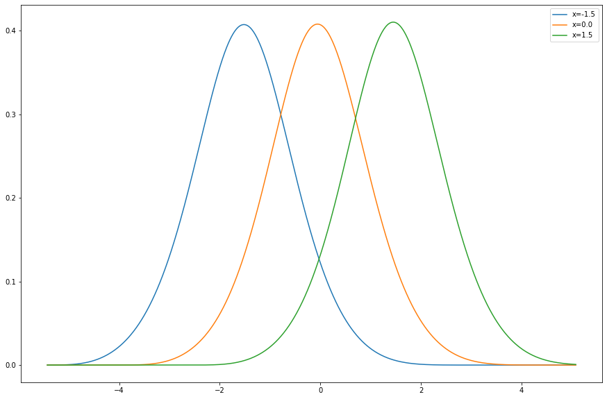
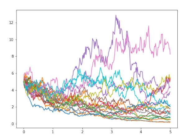
These Markov models are useful in modeling random processes whose current state depends only on the previous state. Below is the process \(X_n=Z_n-X_{n-1}\) where \(Z_n\) are i.i.d. standard normal random variables.
In this project, we first define (for arbitrary dimension \(\mathcal{X}\subset \mathbf{R}^{e_0}\) and customizable network length/depth) an initial law by modeling the CDF of a random variable and then differentiating that to obtain a density function:
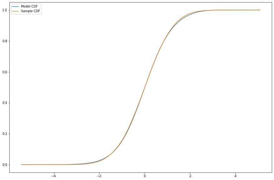
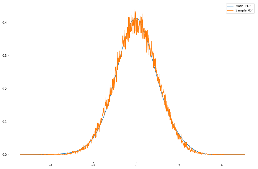
We minimize the cross entropy \(-\mathbf{E}_{dq}[\log(d\mu)] \) to minimize the KL-divergence between the two distributions. We then use this initial law to minimize the KL-divergence between the joint probability measure on 1-jumps in \(\mathcal{X}\times\mathcal{X}\) and the kernel times the initial law \(k(y|x)p(x)\). We obtain \(k\) from differentiating a more complicated Neural Network we call a G-model. This produces a Markov kernel function on \(\mathcal{X}\times\mathcal{X}\):
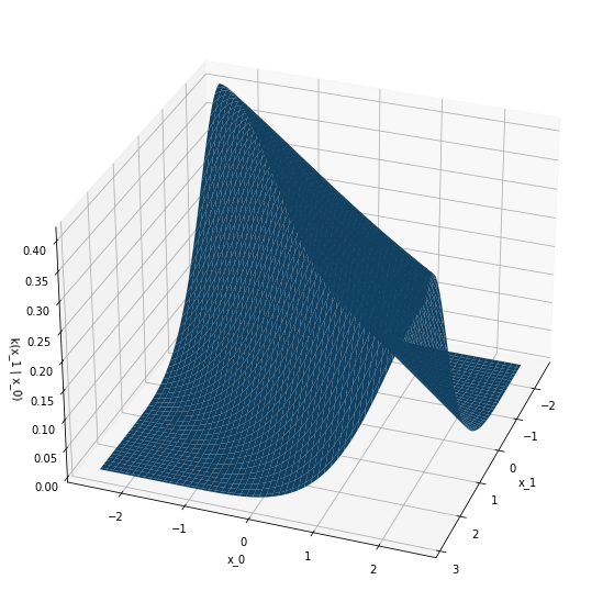
The images above are the results of training the model on samples of simple Gaussian kernel processes:
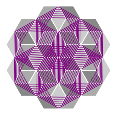
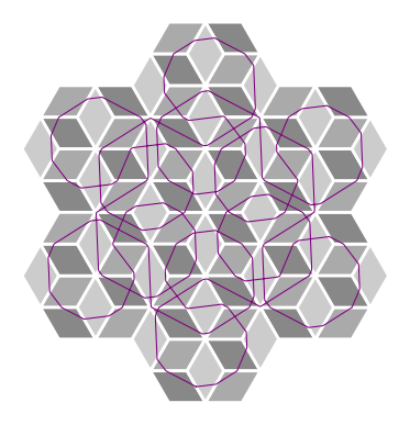
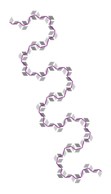
Necker Cube Surface

The Necker cube surface is an infinite periodic Euclidean cone surface homeomorphic to the plane which is tiled by squares meeting three or six to a vertex. The Necker cube surface depicted below is a variant of a family of famous illusions due to Swiss crystallographer Louis A. Necker. However, the pattern has been used as a tiling pattern (called the rhombile tiling) for floors since the ancient Greeks. Afterwards, the surface received a brief mention in Popular Science Monthly in 1899, in an article called The "Mind's Eye" exhibiting a variety of optical illusions. This periodic pattern can be spotted in numerous works by M.C. Escher, and is the game board in the cabinet arcade classic, Q*bert. The illusion of cubes that may alternately be seen as popping in or out of the page captured the interest of people throughout the millennia, but has rarely been considered an object of mathematical study. Its geometric structure, when realized as a flat surface, reveals a deep connection between the symmetries of the surface and the dynamics of its geodesic flow. A paper of mine and Dr. Pat Hooper's that fully characterizes the dynamics of the geodesic flow can be found here: ArXiv:2310.03115. We prove that there is a countable, dense set of directions that are periodic and drift periodic characterized entirely by the parities of trajectory's "slope" components. We also prove results surrounding ergodicity, diffusion, and closed trajectory symmetries.
Pictured below are some examples of geodesics on this surface of slopes 71/73,15/13, and 4/11, in that order. See if you can figure out what about these slopes determines whether the trajectory closes or drifts forever.
To learn about how we got these images, I put together a SAGE jupyter notebook file here and a pdf of it here. Note that you absolutely need to have flatsurf installed in order to make this work. For instructions on how to get flatsurf installed on your specific operating system, check out this informative link on Dr. Pat Hooper's website.
Brauer Algebra Idempotents
As part of my summer internship in 2019, I worked with Dr.Zajj Daugherty to implement the idempotents of the semisimple Brauer Algebra by way of combinatorial representation theory. I've split up the work into three parts as individual SAGE jupyter notebooks. Part 1 introduces the reader to the basic objects of study and tries to motivate the use of the double centralizer theorem to characterize algebra modules. Part 2 looks to use the already implemented symmetric group algebra idempontents to decompose a self-tensored vector space. And finally, Part 3 implements well-known combinatorial methods to calculate and verify idempotents of the semisimple Brauer algebra (for nice deformation parameters). The three parts have been combined and exported to a pdf document here.
For those interested in working on the implementation as an object call in SAGE, a github ticket exists here. I would also like to remark that these idempotents allow us to easily work out a decomposition into sums of copies of isotypic components by passing them through a representation, and determining the rank of the matrix. These idempotents then project onto some multiple of an irreducible algebra module. For those interested in the Kronecker Coefficient Problem, note that the Partition Algebra centralizes the Symmetric Group Algebra. As per Schur-Weyl duality, this means that the dimensions of the Partition algebra corresponding to a particular idempodent are dual to the multiplicities of the irreducible symmetric group component in the tensor product decomposition. By computing these values in Sage, we would obtain far more data to fully tackle the problem. These ideas can be traced back to the following paper by Bowman, De Visscher, and Orellana.
Horseshoes, And Their Spectra
The horseshoe map was introduced by Stephen Smale, and is one of the most famous examples of an invertible, differentiable, two-dimensional chaotic system whose invariant set is conjugate to the two-sided shift map of two symbols. It has since been generalized and certain regularity assumptions have been tested relentlessly. Here is an example of a linear horseshoe of three symbols:
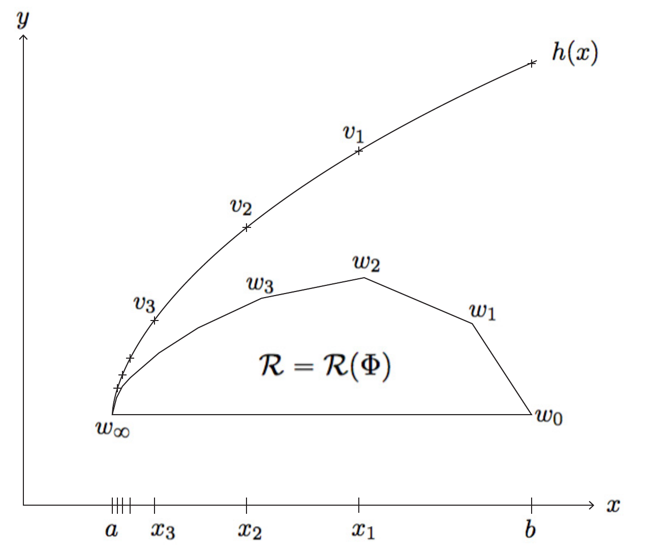
The invariant set of such a map has a "tangent space" that can be decomposed into a sum of stable (horiztonal) and unstable (vertical) vector fields that are preserved by the derivative of the map (always a diagonal matrix). The Lyapunov exponents restricted to these stable and unstable spaces (rate of separation of infinitesimally close trajectories) of the map are therefore entirely determined by the absolute value of these diagonal entries. The set of all such exponents are thus a point in the plane. When we further generalize and allow piecewise linearity of the horseshoe, we get a convex spectra of exponenents in the plane. We call this set the Lyapunov spectrum of the map. If we consider the set M of (Borel) invariant probability measures (measures that are preserved by the horseshoe map and acts as a probability measure on the invariant set), we can measure the integral (w.r.t. the measure) of the logarithm of the absolute value of the derivatives restricted to these subspaces and obtain a point in the plane called a rotation vector. This is the generalization of the Lyapunov spectrum that produces the same convex set for piecewise linear horseshoes. We call this the rotation set, R.
The entropy spectrum of the horseshoe is defined as the supremum of measure-theoretic entropies of the horseshoe that attains a particular rotation vector in R. For a horsehoe map that is Holder with coefficient greater than 1, this coincides with the definition of topological entropy of the map restricted to the points in the system that attain this Lyapunov exponent. This is an important form of dissecting a hyperbolic system into its most primitive components and classification of such systems.
Its known that this entropy spectrum map is continuous on the interior of the Lyapunov spectrum. And, in the case of a piecewise linear horseshow, it is continuous on its boundary as well. What is unknown is whether there exists a horseshoe whose entropy spectrum is discontiniuous on the boundary of the rotation set. Using regularity results of the horseshoe, Christian Wolf, Joe Winters, and I build a recursive sequence of piecewise linear horseshoes that converges to a twice-differentiable, nonlinear dynamical system with all of the same topological properties through a series of local perturbations or "surgeries". However, the spectrum of Lyapunov exponenents is obtained as the convex hull of countably many extrema (with a new extrema added with every iteration). We fix one extreme point to have positive topological entropy (corresponds to a subshift of finite type), and show that the entropy of the additional extremal points are all zero. This produces a theoretical horseshoe with a discontinuous entropy spectrum. The paper can be found here: ArXiv:1910.05837.
Linear Stochastic Differential Equations in Python
As an adaption of Dr. Jay Jorgenson's MATLAB codes, I wanted to see if I could get some quick and dirty python versions of an introductory example to the topic of stochastic differential equations. Click for the notebook file, or the exported pdf. This does not require SAGE to run, and can be easily adapted to nonlinear equations.